Radical Pair Basics & Hamiltonian
The Singlet–Triplet (ST) Basis
\[
\begin{align*}
|S\rangle & = \tfrac{1}{\sqrt{2}}\big(|\uparrow\downarrow\rangle-|\downarrow\uparrow\rangle\big), \\
|T_{+}\rangle &=|\uparrow\uparrow\rangle, \\
|T_0\rangle & = \tfrac{1}{\sqrt{2}}\big(|\uparrow\downarrow\rangle+|\downarrow\uparrow\rangle\big), \\
|T_{-}\rangle &=|\downarrow\downarrow\rangle.
\end{align*}
\]
\(\mathbf{S}_1 \cdot \mathbf{S}_2\) Operator and Projectors
The operator \(\hat{\mathbf{S}}_1 \cdot \hat{\mathbf{S}}_2 = \tfrac{1}{2}(\hat{\mathbf{S}}^2-\hat{\mathbf{S}}_1^2-\hat{\mathbf{S}}_2^2)\) yields eigenvalues of \(-\frac{3}{4}\) for the singlet state and \(+\frac{1}{4}\) for triplet states (with \(\hbar=1\)). This allows us to define the projection operators:
\[
\begin{align*}
\hat{P}_S & = |S\rangle\langle S| = \tfrac{1}{4}\mathbb{1} - \hat{\mathbf{S}}_1 \cdot \hat{\mathbf{S}}_2, \\
\hat{P}_T & = \mathbb{1} - \hat{P}_S = \tfrac{3}{4}\mathbb{1} + \hat{\mathbf{S}}_1 \cdot \hat{\mathbf{S}}_2.
\end{align*}
\]
The Radical Pair Hamiltonian
\[
\hat{H}_{\text{total}} = \underbrace{\hat{H}_{\text{Z}}}_{\text{Zeeman}} + \underbrace{\hat{H}_{\text{H}}}_{\text{Hyperfine}} + \underbrace{\hat{H}_{\text{J}}}_{\text{Exchange}} + \underbrace{\hat{H}_{\text{D}}}_{\text{Dipolar}} + \underbrace{\hat{H}_{\text{K}}}_{\text{Reaction}}
\]
\[
\begin{align*}
\hat{H}_{\text{Z}} & = -\gamma_e \mathbf{B}^{\top} \cdot \sum_{i=1}^{2}\hat{\mathbf{S}}_i - \sum_{i=1}^{2}\sum_{j=1}^{N_i}\gamma^{(n)}_{i,j} \mathbf{B}^{\top} \cdot \hat{\mathbf{I}}_{i,j}, \\
\hat{H}_{\text{H}} & = \sum_{i=1}^{2}\sum_{j=1}^{N_i}\hat{\mathbf{S}}_i^{\top} \cdot \mathbf{A}_{i,j} \cdot \hat{\mathbf{I}}_{i,j}, \\
\hat{H}_{\text{J}} & = -2J \hat{\mathbf{S}}_1^{\top} \cdot \hat{\mathbf{S}}_2, \\
\hat{H}_{\text{D}} & = \hat{\mathbf{S}}_1^{\top} \cdot \mathbf{D} \cdot \hat{\mathbf{S}}_2, \\
\hat{H}_{\text{K}} & = -\tfrac{i}{2}\big(k_S \hat{P}_S + k_T \hat{P}_T\big). \quad\text{(Haberkorn Model)}
\end{align*}
\]
- \(\hat{\mathbf{S}}_i = [\hat{S}_i^x, \hat{S}_i^y, \hat{S}_i^z]\): spin of electron \(i\); \(\hat{\mathbf{I}}_{i,j} = [\hat{I}_{i,j}^x, \hat{I}_{i,j}^y, \hat{I}_{i,j}^z]\): spin of \(j\)-th nucleus coupled to electron \(i\).
- \(\mathbf{A}_{i,j}\): hyperfine tensor; \(\mathbf{D}\): dipolar tensor; \(J\): exchange coupling
- \(k_S, k_T\): spin-selective reaction rates.
Gyromagnetic Ratios & Spin Quantum Numbers
| Electron \(e^-\) |
\(S=1/2\) |
\(-1.76 \times 10^{11}\) |
negative sign |
| \(^{1}\mathrm{H}\) |
\(I=1/2\) |
\(2.68 \times 10^8\) |
Proton |
| \(^{14}\mathrm{N}\) |
\(I=1\) |
\(1.93 \times 10^7\) |
Three levels (\(2I+1=3\)) |
| \(^{13}\mathrm{C}\) |
\(I=1/2\) |
\(6.73 \times 10^7\) |
(\(^{12}\mathrm{C}\) is spin-0) |
- The electron gyromagnetic ratio \(\gamma_e\) is $$1000 times larger than that of nuclei.
- Nuclear-nuclear spin interactions are negligible on the microsecond timescale.
- The Earth’s magnetic field (\(\sim 0.05~\mathrm{mT}\)) induces a tiny electronic Zeeman splitting (\(\sim 70~\mu\text{K}\)).
- EPR experiments are typically conducted at much higher fields (\(\sim 1~\mathrm{T}\)).
Electron–Electron Coupling: \(\mathbf{C} = \mathbf{D} - 2J\mathbb{1}\)
The total spin-spin interaction can be written as:
\[
\hat{H}_{\text{SS}} = \hat{\mathbf{S}}_1^{\top} \mathbf{C} \hat{\mathbf{S}}_2 = \hat{\mathbf{S}}_1^{\top} \mathbf{D} \hat{\mathbf{S}}_2 - 2J \hat{\mathbf{S}}_1 \cdot \hat{\mathbf{S}}_2
\]
- Exchange (\(J\)): Arises from the exchange integral. It determines the singlet-triplet energy gap, \(\Delta E_{ST}=2J\). It typically decays exponentially with inter-radical distance: \(J(r) \approx J_0 e^{-r/a}\).
- Dipolar Tensor (\(\mathbf{D}\)): A through-space magnetic dipole-dipole interaction. It lifts the degeneracy of the triplet sublevels (zero-field splitting). In the point-dipole approximation: \[
\mathbf{D} = \frac{\mu_0}{4\pi} \frac{(\gamma_e\hbar)^2}{r^3} \big(\mathbb{1} - 3\hat{\mathbf{r}}\hat{\mathbf{r}}^{\top}\big)
\] \(|\mathbf{D}|\) decays as \(r^{-3}\), dominating over \(J\) at long range.
The Magnetic Field Effect (MFE)
![]()
- Hyperfine-driven \(S \leftrightarrow T\) interconversion is modulated by the external field \(\mathbf{B}\) (both its magnitude and orientation).
- Since recombination rates are spin-dependent (e.g., the singlet state recombines faster), the overall product yield becomes sensitive to the magnetic field. \[
\Phi_S(\mathbf{B}) = k_S \int_{0}^{\infty} dt\, \mathrm{Tr}\big[\rho(t;\mathbf{B})\,\hat{P}_S\big].
\]
The Liouville-von Neumann Equation
The Density Operator (Statistical Mixture of Nuclear Spin States)
\[
\rho = \sum_{p} w_p |\psi_p\rangle\langle\psi_p|, \quad \text{with } w_p \ge 0, \sum_p w_p = 1.
\]
For a pure state, \(\rho=|\psi\rangle\langle\psi|\) (single wavefunction).
From the Schrödinger equation, \(i\hbar \frac{d}{dt}|\psi\rangle = H |\psi\rangle\), we can derive the equation of motion for the density operator:
\[
\frac{d\rho}{dt} = -\frac{i}{\hbar}[H, \rho]
\]
The solution, \(\rho(t) = U(t)\rho(0)U^\dagger(t)\), represents a completely positive and trace-preserving (CPTP) map, ensuring the physicality of the density operator at all times.
Efficient Computation via Liouville-Space Vectorisation
Start with the full Liouville-von Neumann equation including reaction terms:
\[
\dot{\rho} = -i[H,\rho] - \frac{k_S}{2}\{P_S,\rho\} - \frac{k_T}{2}\{P_T,\rho\}.
\]
Vectorisation reshapes operators into vectors in a “doubled” state space:
\[
\rho \mapsto |\rho\rangle\rangle \in \mathcal{H} \otimes \mathcal{H}, \quad \text{where } \mathrm{vec}(A\rho B)=(B^{\top} \otimes A)|\rho\rangle\rangle.
\]
The equation of motion becomes a linear differential equation:
\[
i\,\partial_t |\rho\rangle\rangle = \hat{\hat{L}}_0 |\rho\rangle\rangle, \quad \text{with }
\hat{\hat{L}}_0 = \mathbb{1} \otimes H - H^{\top} \otimes \mathbb{1} - \frac{i}{2}\sum_{A=S,T} (P_A \otimes \mathbb{1} + \mathbb{1} \otimes P_A^{\top}).
\]
Evaluating \(\langle P_S(t)\rangle\) via spin coherent states
\[
\langle P_S(t)\rangle \;=\; \mathrm{Tr}\!\left[P_S\,\rho(t)\right],\quad
\rho(t)=U(t)\rho(0)U^\dagger(t).
\]
The spin coherent states \(|\Omega_k\rangle = |\theta_k, \phi_k\rangle = (1+|\zeta_k|^2)^{-I_k} e^{\zeta_k \hat{I}_{-}} |m_z=I_k\rangle\), where \(\zeta_k = e^{i \phi_k} \tan(\theta_k/2)\), obey the resolution of identity:
\[
\bigotimes_{k=1}^{N_{\rm nuc}}\!\mathbb{1}_k \;=\;
\bigotimes_{k=1}^{N_{\rm nuc}}
\frac{2I_k+1}{4\pi}
\int_0^{2\pi} d\phi_k \int_0^{\pi} d\theta_k \sin(\theta_k)
|\Omega_k\rangle\!\langle\Omega_k|.
\]
At room temperature one often has \(\rho(0)\propto P_S\otimes \mathbb{1}_{\rm nuc}\), giving
\[
\langle P_S(t)\rangle \;=\; \int \! d\boldsymbol{\Omega}\; p(\boldsymbol{\Omega})\;
\langle S, \boldsymbol{\Omega} | U^\dagger(t) P_S U(t) | S, \boldsymbol{\Omega} \rangle.
\]
Spin coherent state basis \(|\boldsymbol{\Omega}\rangle\) converges faster than the product basis \(|\mathbf{m}\rangle\) in the stochastic Schrödinger equation.
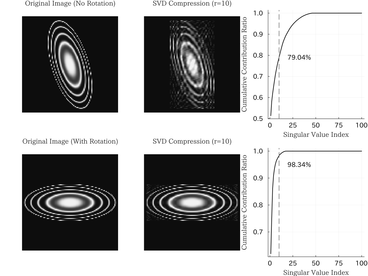
Low-Rank Approximation via SVD
Best Rank-\(r\) Approximation
For any matrix \(X\), the singular value decomposition (SVD) is \(X = U\Sigma V^\dagger\). The best rank-\(r\) approximation to \(X\) is found by keeping only the \(r\) largest singular values:
\[
X_r = \sum_{i=1}^{r} \sigma_i \mathbf{u}_i \mathbf{v}_i^\dagger \quad (r < \mathrm{rank}(X))
\]
This truncation minimises the Frobenius norm of the error on the low-rank manifold \(\mathcal{M}_r=\{Y:\,\mathrm{rank}(Y)\le r\}\):
\[
X_r = \arg\min_{Y \in \mathcal{M}_r} \| X - Y \|_F
\]
The largest singular values capture the main features of the matrix. Discarding small ones compresses the data, as in image compression and tensor networks.
SVD as Image Compression
![]()
Diagrammatic Tensor Notation
We can represent tensors graphically to make complex contractions intuitive.
- A node represents a tensor.
- A leg (or edge) represents an index.
- Connecting legs implies summation over the shared index (contraction).
![]()
SVD as a Tensor Network: A matrix (rank-2 tensor) is decomposed into a chain of three tensors.
![]()
Matrix Product States (MPS)
A many-body quantum state can be efficiently represented by factorising its coefficient tensor into a one-dimensional chain of smaller tensors:
\[
|\Psi\rangle = \sum_{\sigma_1,\dots,\sigma_N}
A^{[1]}_{\sigma_1}
A^{[2]}_{\sigma_2}\cdots
A^{[N]}_{\sigma_N}
|\sigma_1, \dots, \sigma_N\rangle
\]
![]()
- The dimensions of the connecting “virtual” bonds, known as the bond dimension, control the accuracy of the approximation.
- This representation is close to exact for states with low entanglement.
- We use this for the stochastic Schrödinger approach, where each trajectory \(|\Psi_p(t)\rangle\) is an MPS.
Matrix Product Operator (MPO)
MPO from sum of products of local operators (such as \(S_x\))
\[
\hat{H} = \sum_{\{\sigma_k^\prime, \sigma_k\}}
\prod_{k=1}^{N} \hat{W}^{[k]}, \quad
\hat{W}^{[k]} = W_{\sigma_k^\prime, \beta_{k-1} \beta_k, \sigma_k} |\sigma_k^\prime\rangle \langle\sigma_k|
\]
The tensor elements \(W_{\sigma_k^\prime, \beta_{k-1} \beta_k, \sigma_k} \in \mathbb{C}^{M_{k-1} \times d_k \times d_k\times M_k}\) are determined by bipartite graph theory [Ren et al. (JCP, 2020)].
![]()
Vectorised MPDO (vMPDO)
Liouville-space equation (bond dimension \(\boldsymbol{\chi}\))
\[
i\frac{d}{dt}|\rho\rangle\rangle
= \hat{\hat{L}}_0 |\rho\rangle\rangle,\quad
\hat{\hat{L}}_0=\mathbb{1}\!\otimes \hat{H}-\hat{H}^{\top}\!\otimes\mathbb{1}
-\frac{i}{2}\sum_{X=S,T}\!\left(\hat{P}_X\!\otimes\!\mathbb{1}+\mathbb{1}\!\otimes\!\hat{P}_X^{\top}\right).
\]
![]()
The Purification Approach (LPMPS)
Physical density operator (bond dimension \(\mathbf{r}\))
The physical density operator is recovered by tracing out an ancilla system:
\[
\rho_{\text{phys}}(t) = \mathrm{Tr}_{\text{anc}}\left( |\Psi_{\text{pur}}(t)\rangle\langle\Psi_{\text{pur}}(t)| \right)
\]
\[
|\Psi_{\mathrm{pur}}\rangle
=\!\!\sum_{\{\sigma_k,s_k\}}\!
\Big(\prod_{\ell=1}^{2N} A^{[\ell]}_{\xi_\ell}\Big)\,
|\xi_1,\ldots,\xi_{2N}\rangle,\quad
\xi_{2k-1}=\sigma_k,\;\xi_{2k}=s_k
\]
- The total system (physical + ancilla) is represented by a single pure-state MPS.
- Time evolution is performed with the physical Hamiltonian acting only on the physical sites: \(\hat{H}_{\text{total}} = \hat{H}_{\text{phys}} \otimes \mathbb{1}_{\text{anc}}\).
Refs: Verstraete et al. (PRL, 2004)
LPMPS
![]()
Complete positivity (CP)
Let \(U_{\mathrm{tot}}(t)=e^{-i(H_{\mathrm{phys}}\otimes \mathbb{1})t}\). Then
\[
\rho(t)=\mathrm{Tr}_{\mathrm{anc}}\!\left[U_{\mathrm{tot}}(t)\,
|\Psi_{\mathrm{pur}}(0)\rangle\langle\Psi_{\mathrm{pur}}(0)|\,
U_{\mathrm{tot}}^\dagger(t)\right]
=U_{\mathrm{phys}}(t)\,\rho(0)\,U_{\mathrm{phys}}^\dagger(t),
\]
which is nothing other than the time evolution of the physical density operator.
By definition, \(\rho(t) = |\Psi_{\mathrm{pur}}(t)\rangle\langle\Psi_{\mathrm{pur}}(t)|\), density operator holds the semidefinite property.
![]()
Key Advantage: Guaranteed Positivity
Since the resulting \(\rho_{\text{phys}}(t)\) is obtained by partially tracing a pure state, it is guaranteed to be a positive semidefinite operator by construction, a crucial physical property that can be violated in the vMPDO approach if the bond dimension is too small.
Summary of Tensor Network Methods
| Space |
Hilbert |
Liouville |
Hilbert+Ancilla |
| State |
Ensemble of \(|\Psi_p\rangle\) |
\(|\rho\rangle\rangle\) |
Single \(|\Psi_{\text{pur}}\rangle\) |
| Linear Action |
\(\hat{H}\) |
\(\hat{\hat{L}}\) |
\(H_{\mathrm{phys}}\otimes \mathbb{1}_{\mathrm{anc}}\) |
| Bond Dim. |
\(m\) |
\(\chi\) |
\(r\) |
| Cost |
\(\mathcal{O}(K N m^3)\) |
\(\mathcal{O}(N \chi^3)\) |
\(\mathcal{O}(N r^3)\) |
| Deterministic? |
No |
Yes |
Yes |
| Guaranteed Positivity? |
Yes |
No |
Yes |
| Parallelisation |
Distributed Memory |
Shared Memory |
Shared Memory |
- Stochastic MPS: Requires many trajectories (\(K\)) but often with a smaller bond dimension (\(m\)) per trajectory. Excellent for parallel computing.
- vMPDO/LPMPS: Deterministic but require larger bond dimensions (\(\chi, r\)) and more memory, making them suitable for powerful single-node or shared-memory systems.
Time Evolution via the Time-Dependent Variational Principle (TDVP)
Applying the time evolution operator \(e^{-i\hat{H}\Delta t}\) to an MPS generally increases its bond dimension. To keep the simulation tractable, we must project the evolved state back onto the low-rank MPS manifold.
TDVP provides a principled way to perform this projection. It approximates the exact time evolution by finding the optimal state within the MPS manifold at each timestep.
\[
\frac{d}{dt}|\Psi(t)\rangle = -i \mathcal{P}_{\mathcal{T}}\left( \hat{H}|\Psi(t)\rangle \right)
\]
where \(\mathcal{P}_{\mathcal{T}}\) projects onto the tangent space of the MPS manifold.
Refs: Haegeman et al. (PRB, 2016)
Magnetosensitivity of Quantum Birds
The Radical Pair Hypothesis of Avian Magnetoreception
A light-activated radical pair, formed in cryptochrome proteins in a bird’s retina, acts as a chemical magnetic compass.
- The Earth’s magnetic field affects the S-T conversion rate, changing the amount of signalling product formed.
- The bird perceives this change as a visual pattern, allowing it to “see” the magnetic field lines.
- Magnetic sensitivity of cryptochrome 4 (CRY4) from the European robin has been demonstrated experimentally (Xi et al, Nature 2021).
YouTube: https://youtu.be/0SPD2r0xV8k
Application: Flavin–Tryptophan Radical Pair in CRY4
We model the FAD\(^{\bullet-}\) – TrpH\(^{\bullet+}\) radical pair in avian cryptochrome, using realistic, anisotropic hyperfine and electron-electron couplings.
![]()
The flavin (FAD) and tryptophan (Trp) molecules involved in the radical pair.
Kinetic scheme of cryptochrome radical pairs (cartoon)
![]()
Refs: Xu et al. (Nature 2021), units are in \(\mathrm{s}^{-1}\)
Modelling Electron Hopping Between Two Radical Pairs
In cryptochrome, the electron hole can hop between different tryptophan residues, creating a network of radical pairs (e.g., RP\(_C\) and RP\(_D\)).
- We model the dynamics of two coupled radical pairs (FAD/TrpC and FAD/TrpD) sharing a common flavin.
- The hopping electron site is described by
\[
\begin{gathered}
\mathrm{span}\{|\uparrow\uparrow 0\rangle, |\uparrow\downarrow 0\rangle, |\downarrow\uparrow 0\rangle, |\downarrow\downarrow 0\rangle, |\uparrow 0 \uparrow\rangle, |\uparrow 0 \downarrow\rangle, |\downarrow 0 \uparrow\rangle, |\downarrow 0 \downarrow\rangle\} \\
= \mathrm{span}\{|T_{+}^{\mathrm{C}}\rangle, |T_0^{\mathrm{C}}\rangle, |S^{\mathrm{C}}\rangle, |T_-^{\mathrm{C}}\rangle, |T_+^{\mathrm{D}}\rangle, |T_0^{\mathrm{D}}\rangle, |S^{\mathrm{D}}\rangle, |T_-^{\mathrm{D}}\rangle\}
\end{gathered}
\]
and Lindblad master equation,
\[
\begin{gathered}
\mathcal{D}[\hat{\rho}] = \sum_{j\in\{\mathrm{C}\to\mathrm{D}, \mathrm{D}\to\mathrm{C}\}} \hat{L}_{j} \hat{\rho} \hat{L}_{j}^\dagger - \frac{1}{2} \hat{L}_{j}^\dagger \hat{L}_{j} \hat{\rho} - \frac{1}{2} \hat{\rho} \hat{L}_{j}^\dagger \hat{L}_{j} \\
\hat{L}_{\mathrm{C}\to \mathrm{D}} = \sqrt{k_{\mathrm{C}\to \mathrm{D}}} \left( |\mathrm{D}\rangle\langle\mathrm{C}|\right), \quad
\hat{L}_{\mathrm{D}\to \mathrm{C}} = \sqrt{k_{\mathrm{D}\to \mathrm{C}}} \left( |\mathrm{C}\rangle\langle\mathrm{D}|\right)
\end{gathered}
\]
Use \(\mathrm{vec}(A\rho B)=(B^\top\!\otimes A)|\rho\rangle\rangle\) to build \(\hat{\hat{L}}\) and evolve as MPS.
Hamiltonian parameters
Hamiltonian parameters:
- \(J\): exchange coupling taken from experiment by Gravell et al. (JACS, 2025).
- \(J_{C} = 0.011 ~\mathrm{mT}\)
- \(J_{D} = 0.001 ~\mathrm{mT}\)
- \(\mathbf{D}\): dipolar tensor taken from point-dipole approximation and crystal structure
- \(\vec{r}_{C} = (9.480, -13.675, 5.388)\) Å
- \(\vec{r}_{D} = (8.980, -18.684, 4.159)\) Å
\[
\mathbf{D}_{C}-2J_{C}\mathbb{1} =
\begin{pmatrix}
-0.019 & -0.441 & -0.174 \\
-0.441 & -0.311 & 0.251 \\
-0.174 & 0.251 & -0.226
\end{pmatrix}
~\mathrm{mT}
\]
\[
\mathbf{D}_{D}-2J_{D}\mathbb{1} =
\begin{pmatrix}
0.068 & 0.221 & -0.049 \\
0.221 & -0.286 & 0.102 \\
-0.049 & 0.102 & 0.152
\end{pmatrix}
~\mathrm{mT}
\]
- \(\mathbf{A}_{i,j}\): hyperfine tensor taken from electronic structure calculation by ORCA
- \(|B|\): geomagnetic field strength 0.05 mT
Singlet yield
Definition:
\[
\mathbf{B} = B_0 [\cos\theta \cos\phi, \cos\theta \sin\phi, \sin\theta]
\]
We set \(B_0 = 0.05 ~\mathrm{mT}\) and \(\phi = 0\).
\[
\Phi_S(\tau; \theta) = k_S \int_{0}^{\tau} \! dt~\mathrm{Tr}\!\left[\rho(t; \theta)\,\hat{P}_S\right].
\]
Anisotropic Magnetosensitivity at 0.05 mT with limited nuclear spins
The relative change in singlet yield, \(\Phi_S\), as a function of the magnetic field orientation (\(\theta\)).
Anisotropic magnetosensitivity at 0.05 mT
Up to 30 nuclear spins.
Time-dependence of \(\Phi_S(\tau; \theta)\) changes. only 0.06 % anisotropy
Anisotropic Magnetosensitivity at 5.0 mT (100 \(\times\) higher)
- The anisotropy is now much larger (\(\sim 5\%\)).
- The orientation is completely different from low-field case.