Fitting of 2D PES

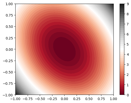
In this case, we consider PES written by \[ V(x,y) = 4x^2 + 3y^2 + 2xy \]

Code

import platform
import sys

import pompon

print(sys.version)
print(f"pompon version = {pompon.__version__}")
print(platform.platform())

3.12.2 (main, Feb  6 2024, 20:19:44) [Clang 15.0.0 (clang-1500.1.0.2.5)]
pompon version = 0.0.9
macOS-14.4.1-arm64-arm-64bit

Code

import jax.numpy as jnp
import matplotlib.pyplot as plt
import numpy as np
from tqdm.auto import tqdm

from pompon.layers.tensor import TwodotCore
from pompon.utils import train_test_split

Code

def ellipse_pes(
    x: np.ndarray | float, y: np.ndarray | float
) -> np.ndarray | float:
    return 4.0 * x**2 + 3.0 * y**2 + 2.0 * x * y

Code

def plot_ellipse():
    x = np.linspace(-1, 1, 100)
    y = np.linspace(-1, 1, 100)
    X, Y = np.meshgrid(x, y)
    Z = ellipse_pes(X.flatten(), Y.flatten()).reshape(X.shape)
    plt.contourf(X, Y, Z, 50, cmap="RdGy", vmax=9, vmin=0)
    plt.colorbar()
    plt.show()

Code

plot_ellipse()

Sampling from Boltzman distribution \(\exp(-\beta V)\) is anallytically achievable by using multivariate normal distribution.

Code

def sample_ellipse(
    N: int = 100, β: float = 1.0e01
) -> tuple[np.ndarray, np.ndarray]:
    # sample from a 2D Gaussian
    np.random.seed(0)
    A = np.array([[4, 1], [1, 3]])
    # Σ^-1 / 2 = A * β
    Σ = np.linalg.inv(A * β * 2.0)
    μ = np.array([0, 0])
    x = np.random.multivariate_normal(μ, Σ, N)
    return x[:, 0], x[:, 1]

Code

x = np.linspace(-1, 1, 100)
y = np.linspace(-1, 1, 100)
X, Y = np.meshgrid(x, y)
Z = ellipse_pes(X.flatten(), Y.flatten()).reshape(X.shape)
plt.contourf(X, Y, Z, 20, cmap="RdGy", vmax=9, vmin=0)
plt.colorbar()
x, y = sample_ellipse(N=100, β=1.0e01)
plt.scatter(x, y, label="β=1.e+01")
x, y = sample_ellipse(N=100, β=1.0e00)
plt.scatter(x, y, label="β=1.e+00")
plt.legend()
plt.show()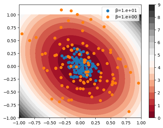

One constructs following NNMPO

Code

N = 20  # Number of basis per site
M = 1  # Bond dimension
nnmpo = pompon.model.NNMPO(
    input_size=2,
    hidden_size=2,
    basis_size=N,
    bond_dim=M,
    activation="silu",
)

You can change activation. See pompon.layers.activations for available activations.

Sample 256 points with temperature β=1.0

Code

x, y = sample_ellipse(N=256, β=1.0e00)
x = np.stack([x, y], axis=1)
y = ellipse_pes(x[:, 0], x[:, 1]).reshape(-1, 1)
x_train, x_validate, y_train, y_validate = train_test_split(
    x, y, train_size=0.7
)
print(x_train.shape)
print(y_train.shape)

(179, 2)
(179, 1)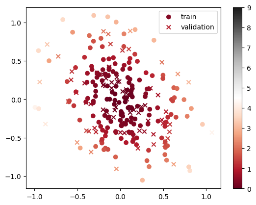

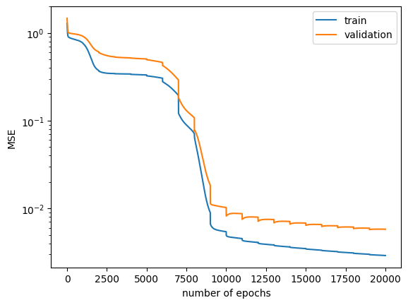
Code

y_pred = nnmpo.forward(x_train)
print(y_pred.shape)

(179, 1)

Code

plt.scatter(
    x_train[:, 0],
    x_train[:, 1],
    c=y_train[:, 0],
    label="train",
    cmap="RdGy",
    vmax=9,
    vmin=0,
    marker="o",
)
plt.scatter(
    x_validate[:, 0],
    x_validate[:, 1],
    c=y_validate[:, 0],
    label="validation",
    cmap="RdGy",
    vmax=9,
    vmin=0,
    marker="x",
)
plt.colorbar()
plt.legend()
plt.show()

To grasp the optimization routine, one employs manual gradient descent (GD) rather than a trainer.

Code

lr = 1.0e-02
lr_tt = 1.0e-04
train_losses = []
validation_losses = []
tt_rank_epochs = []
norms = []

Code

def evaluate_loss(model, x, y, losses):
    y_pred = model.forward(x)
    loss = pompon.losses.mse(y, y_pred)
    losses.append(loss)
    return loss

Code

for i_epoch in tqdm(range(20_000)):
    evaluate_loss(nnmpo, x_train, y_train, train_losses)
    evaluate_loss(nnmpo, x_validate, y_validate, validation_losses)
    params = nnmpo.grad(
        x_train, y_train, basis_grad=True, coordinator_grad=True
    )
    for param in params:
        param.data -= lr * param.grad
    if (i_epoch + 1) % 1_000 == 0:
        nnmpo.update_blocks_batch(x_train)
        for _ in tqdm(range(5_000)):
            params = nnmpo.grad(
                x_train, y_train, twodot_grad=True, to_right=True
            )
            B: TwodotCore = params[0]
            B.data -= lr_tt * B.grad
        nnmpo.tt.norm.data *= (norm := jnp.linalg.norm(B.data))
        B.data /= norm
        W0, W1 = B.svd(truncation=0.99, rank=2)
        nnmpo.tt.W0.data = W0.data
        nnmpo.tt.W1.data = W1.data
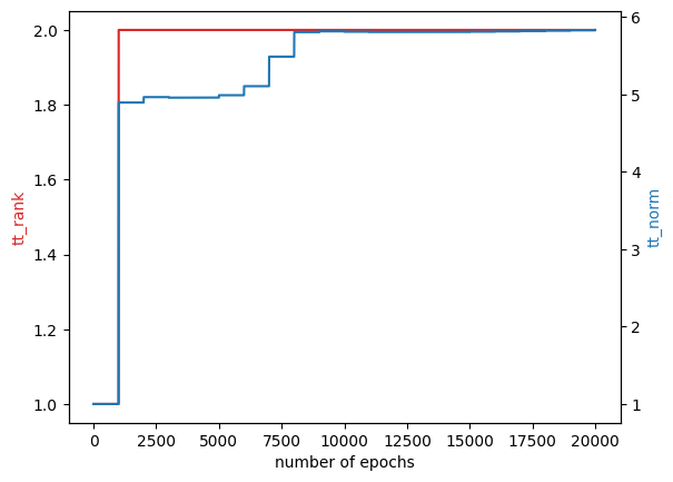
    norms.append(nnmpo.tt.norm.data)
    tt_rank_epochs.append(nnmpo.tt.ranks)

Explanation of the code:

Lines 1~3:

for i_epoch in tqdm(range(20_000)):
   evaluate_loss(nnmpo, x_train, y_train, train_losses)
   evaluate_loss(nnmpo, x_validate, y_validate, validation_losses)

Performs training for 20,000 epochs. Calculates Mean Squared Error (MSE) every epoch and logs it.

Lines 4~6:
```
   params = nnmpo.grad(x_train, y_train, basis_grad=True, coordinator_grad=True)
   for param in params:
      param.data -= lr * param.grad
```
Retrieves gradients for parameters \(w\), \(b\), and \(U\) using automatic differentiation and optimizes them using gradient descent. The \(U\) is automatically retracted to the Stiefel manifold by calling - operator.
Lines 7~8:
```
   if (i_epoch +1) % 1_000 == 0:
      nnmpo.update_blocks_batch(x_train)
```
Optimizes Tensor Train (TT) every 1000 epochs. Computes all TT basis for each batch.

Lines 9~12:

      for _ in tqdm(range(5_000)):
          params = nnmpo.grad(x_train, y_train, twodot_grad=True)
          B = params[0] # 
          B.data -= lr_tt * B.grad

Twodot core \(B\) is also optimized by using gradient descent. Here, gradients are calculated analytically.

Lines 13~17:
```
      nnmpo.tt.norm.data *= (norm := jnp.linalg.norm(B.data))
      B.data /= norm
      W0, W1 = B.svd(truncation=0.99, rank=2)
      nnmpo.tt.W0.data = W0.data
      nnmpo.tt.W1.data = W1.data
```
After gradient descent optimization of Twodot core \(B\), Twodot core \(B\) is normalized and decomposed into two Onedot cores \(W\) using Singular Value Decomposition (SVD). It adaptively truncates small singular values and corresponding singular vectors, keeping only the top 99% contribution.

Why did we set rank=2?

The elliptic function has a 3-rank structure. \[ 4x^2 + 3y^2 + 2xy = \begin{bmatrix} 4x^2 & 2x & 1 \end{bmatrix} \begin{bmatrix} 1 \\ y \\ 3y^2 \end{bmatrix} \] However, if coordinator learns low-rank coordinates, \[ [q_1, q_2] = [x, y] U \] where \(U\) diagonalizes the Hessian matrix, \[ A = \begin{bmatrix} 8 & 1 \\ 1 & 6 \end{bmatrix} \] then, the elliptic function becomes \[ 4x^2 + 3y^2 + 2xy = \lambda_1 q_1^2 + \lambda_2 q_2^2 \] where \(\lambda_1\) and \(\lambda_2\) are eigenvalues of \(A\). Thus, we can rewrite the elliptic function as a 2-rank structure. \[ \begin{bmatrix} \lambda_1 & \lambda_2 q_1^2 \\ \end{bmatrix} \begin{bmatrix} q_2^2 \\ 1 \end{bmatrix} \]

Code

plt.plot(train_losses, label="train")
plt.plot(validation_losses, label="validation")
plt.xlabel("number of epochs")
plt.ylabel("MSE")
plt.yscale("log")
plt.legend()
plt.show()

Code

fig, ax1 = plt.subplots()

color = "tab:red"
ax1.set_xlabel("number of epochs")
ax1.set_ylabel("tt_rank", color=color)
ax1.plot(np.array(tt_rank_epochs), color=color)

ax2 = ax1.twinx()
color = "tab:blue"
ax2.set_ylabel("tt_norm", color=color)
ax2.plot(np.array(norms), color=color)

plt.show()

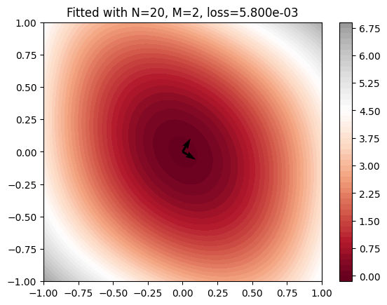
Visualize results

Code

x = np.linspace(-1.0, 1.0, 100)
y = np.linspace(-1.0, 1.0, 100)
X, Y = np.meshgrid(x, y)
Z = nnmpo.forward(jnp.stack([X.flatten(), Y.flatten()], axis=1))[:, 0].reshape(
    X.shape
)
plt.title(
    f"Fitted with N={N}, "
    + f"M={max(tt_rank_epochs[-1])}, "
    + f"loss={validation_losses[-1]:.3e}"
)
plt.contourf(X, Y, Z, 50, cmap="RdGy", vmax=9, vmin=0)
plt.colorbar()
u = nnmpo.coordinator.U.data[0, :]
v = nnmpo.coordinator.U.data[1, :]
plt.quiver(0, 0, u[0], u[1])
plt.quiver(0, 0, v[0], v[1])
plt.show()