Fitting of \(n\)-Dimensional PES

In this example we will consider \[ V(\boldsymbol{x}) = \boldsymbol{x}^\intercal \boldsymbol{A} \boldsymbol{x} \] where \(\boldsymbol{A}\) satisfies \(\det{\boldsymbol{A}}>0\).

Environment

Code

import platform
import sys

import pompon

print(sys.version)
print(f"pompon version = {pompon.__version__}")
print(platform.platform())

3.12.2 (main, Feb  6 2024, 20:19:44) [Clang 15.0.0 (clang-1500.1.0.2.5)]
pompon version = 0.0.9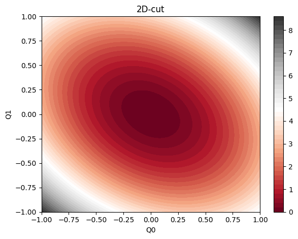
macOS-14.4.1-arm64-arm-64bit

Import modules

Code

import matplotlib.pyplot as plt
import numpy as np

from pompon.utils import train_test_split

Define the potential energy surface

Code

# number of dimension
n = 6

A = np.diag(np.linspace(2.0, 5.0, n))
A += 1.0

print(f"A=\n{A}")
assert np.linalg.det(A) > 0

A=
[[3.  1.  1.  1.  1.  1. ]
 [1.  3.6 1.  1.  1.  1. ]
 [1.  1.  4.2 1.  1.  1. ]
 [1.  1.  1.  4.8 1.  1. ]
 [1.  1.  1.  1.  5.4 1. ]
 [1.  1.  1.  1.  1.  6. ]]

Code

def ellipse_pes(x):
    if x.ndim == 2:
        return np.einsum("Da,ab,bD->D", x, A, x.T)
    else:
        return x @ (A @ x.T)

Code

def ellipse_force(x):
    return -2.0 * x @ A

Code

def plot_2d_cut(dims=(0, 1)):
    # cut of z
    q0 = np.linspace(-1, 1, 100)
    q1 = np.linspace(-1, 1, 100)
    Q0, Q1 = np.meshgrid(q0, q1)
    x = np.zeros((100 * 100, n))
    x[:, dims[0]] = Q0.flatten()
    x[:, dims[1]] = Q1.flatten()
    y = ellipse_pes(x).reshape(Q0.shape)
    plt.clf()
    plt.contourf(Q0, Q1, y, 50, cmap="RdGy", vmax=9, vmin=0)
    plt.xlabel(f"Q{dims[0]}")
    plt.ylabel(f"Q{dims[1]}")
    plt.title("2D-cut")
    plt.colorbar()
    plt.tight_layout()
    plt.show()

Code

plot_2d_cut(dims=(0, 1))

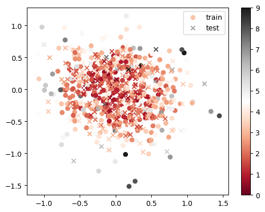
Sampling of learning points

Learning points are sampled from Boltzman distribution \(\exp(-\beta V)\), which is anallytically achievable by using multivariate normal distribution.

Code

def sample_ellipse(N=100, β=1.0e01):
    # sample from a 2D Gaussian
    np.random.seed(0)
    # Σ^-1 / 2 = A * β
    Σ = np.linalg.inv(A * β * 2.0)
    μ = np.zeros(A.shape[0])
    x = np.random.multivariate_normal(μ, Σ, N)
    return x

Code

dims = (0, 1)
q0 = np.linspace(-1, 1, 100)
q1 = np.linspace(-1, 1, 100)
Q0, Q1 = np.meshgrid(q0, q1)
x = np.zeros((100 * 100, n))
x[:, dims[0]] = Q0.flatten()
x[:, dims[1]] = Q1.flatten()
y = ellipse_pes(x).reshape(Q0.shape)
plt.contourf(Q0, Q1, y, 50, cmap="RdGy", vmax=9, vmin=0)
plt.colorbar()
plt.xlabel(f"Q{dims[0]}")
plt.ylabel(f"Q{dims[1]}")


x = sample_ellipse(N=100, β=1.0e01)
plt.scatter(x[:, dims[0]], x[:, dims[1]], label="β=1.e+01")

x = sample_ellipse(N=100, β=1.0e00)
plt.scatter(x[:, dims[0]], x[:, dims[1]], label="β=1.e+00")
plt.legend()
plt.show()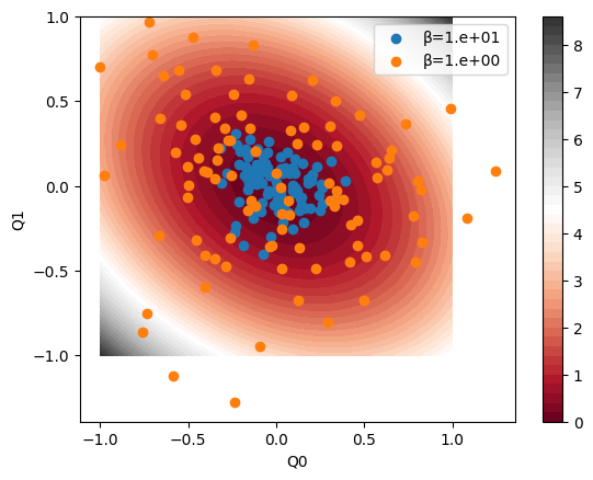

One will sample \(20n^2\) points with temperature \(\beta=1.0\).

Code

x = sample_ellipse(N=20 * (n**2), β=1.0e00)
y = ellipse_pes(x).reshape(-1, 1)
f = ellipse_force(x).reshape(-1, n)
x_train, x_test, y_train, y_test, f_train, f_test = train_test_split(
    x, y, f, train_size=0.7
)
print(x_train.shape)
print(y_train.shape)
print(f_train.shape)

(503, 6)
(503, 1)
(503, 6)

Code

plt.scatter(
    x_train[:, 0],
    x_train[:, 1],
    c=y_train[:, 0],
    label="train",
    cmap="RdGy",
    vmax=9,
    vmin=0,
    marker="o",
)
plt.scatter(
    x_test[:, 0],
    x_test[:, 1],
    c=y_test[:, 0],
    label="test",
    cmap="RdGy",
    vmax=9,
    vmin=0,
    marker="x",
)
plt.colorbar()
plt.legend()
plt.show()

Constructing the data & model

To stabilize the learning, one standardizes the input data.

Code

x_scale = x_train.std()
x_train /= x_scale
x_test /= x_scale
y_shift = y_train.mean()
y_train -= y_shift
y_test -= y_shift
y_scale = y_train.std()
y_train /= y_scale
y_test /= y_scale
f_train *= x_scale / y_scale
f_test *= x_scale / y_scale

Code

N = 20  # Number of basis per site
M = 1  # Initial Bond dimension
nnmpo = pompon.model.NNMPO(
    input_size=n,
    hidden_size=n,
    basis_size=N,
    bond_dim=M,
    activation="moderate+silu",
    b_scale=0.0,
    w_scale=1.0,
    x0=x_train[: N - 1],
)
# nnmpo.fix_bias=True

Code

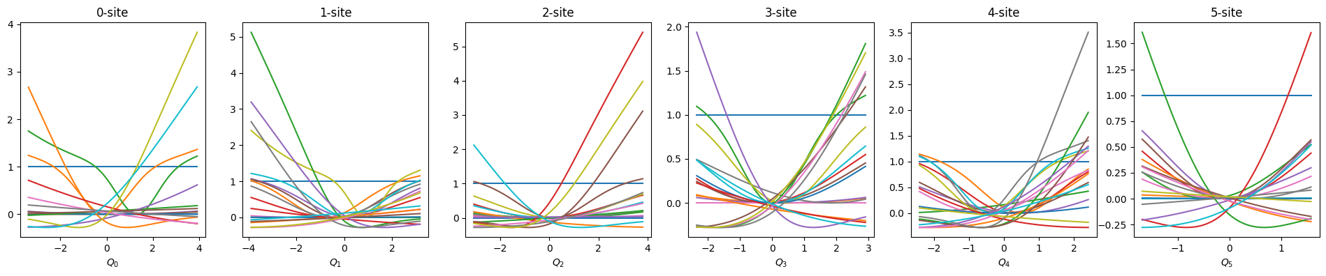
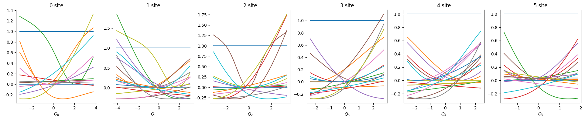
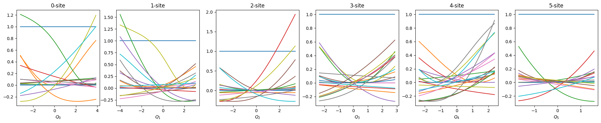
def show_basis(model):
    f = model.hidden_size
    fig, axs = plt.subplots(1, f, figsize=(4 * f, 4))
    q = model.coordinator.forward(x_train)
    q0 = model.q0
    for i in range(f):
        _q = np.linspace(np.min(q[:, i]), np.max(q[:, i]), 100)
        phi = model.basis[i].forward(_q, q0[:, i])
        axs[i].set_title(f"{i}-site")
        axs[i].set_xlabel(f"$Q_{i}$")
        axs[i].plot(_q, phi)
    plt.show()


show_basis(nnmpo)
nnmpo.basis.plot_data()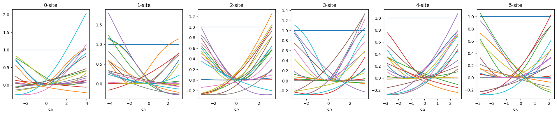

Construct model like this;

Training

Let’s start machine learning!

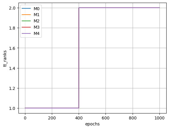
Adam: Adam optimizer
lr: learning rate \(\eta\)
batch_size: Batch size for stochastic gradient descent.
epochs: Number of iterations for optimizing \(w\), \(b\), and \(U\).
nsweeps: Number of sweeps
optax_solver: Solver used for TT optimization
cutoff: Singular value cutoff thereshold
maxdim: Max bond dimension

We know that \[ V(\boldsymbol{x}) = \boldsymbol{x}^\intercal \boldsymbol{A} \boldsymbol{x} \] has 2-rank structure by diagonalizing \(\boldsymbol{A}\), i.e., \[ V(\boldsymbol{x}) = \boldsymbol{x}^\intercal \boldsymbol{U} \boldsymbol{\Lambda} \boldsymbol{U}^\intercal \boldsymbol{x} = \boldsymbol{q}^\intercal \boldsymbol{\Lambda} \boldsymbol{q} = \begin{bmatrix} 1 & \lambda_1 q_1^2 \end{bmatrix} \begin{bmatrix} 1 & \lambda_2 q_2^2 \\ 0 & 1 \end{bmatrix} \cdots \begin{bmatrix} 1 & \lambda_{n-1} q_{n-1}^2 \\ 0 & 1 \end{bmatrix} \begin{bmatrix} \lambda_n q_n^2 \\ 1 \end{bmatrix} \]

Thus, we set maxdim=2.

Code

import optax

from pompon.optimizer import Adam, Sweeper

optimizer = Adam(lr=1.0e-02).setup(
    model=nnmpo,
    x_train=x_train,
    y_train=y_train,
    f_train=f_train,
    batch_size=125,
    x_test=x_test,
    y_test=y_test,
)
sweeper = Sweeper(optimizer)
for i in range(4):
    trace = optimizer.optimize(
        epochs=200,
        epoch_per_log=200,
    )
    show_basis(nnmpo)
    trace = sweeper.sweep(
        nsweeps=4,
        optax_solver=optax.adam(1.0e-03),
        opt_batchsize=10000,
        opt_maxiter=1000,
        opt_tol=1.0e-03,
        cutoff=1.0e-01,
        maxdim=2,
        onedot=(i == 0),
        auto_onedot=True,
    )

# After adam, switch to conjugate gradient.
trace = sweeper.sweep(
    nsweeps=10,
    use_CG=True,
    opt_batchsize=10000,
    opt_maxiter=1000,
    opt_tol=1.0e-10,
    onedot=True,
)
optimizer.lr = 1.0e-05  # reduce learning rate
trace = optimizer.optimize(
    epochs=200,
    epoch_per_log=200,
)

2024-10-16 10:37:11 - INFO:pompon.pompon.model - Model is exported to ./model_initial.h5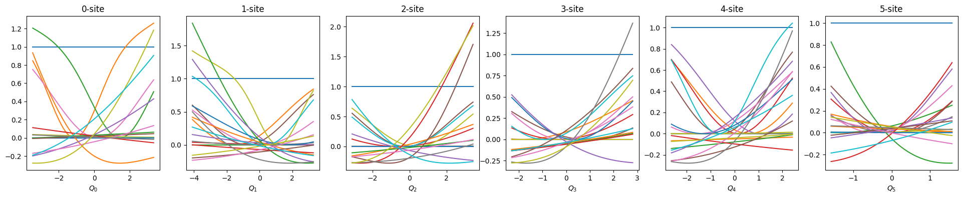

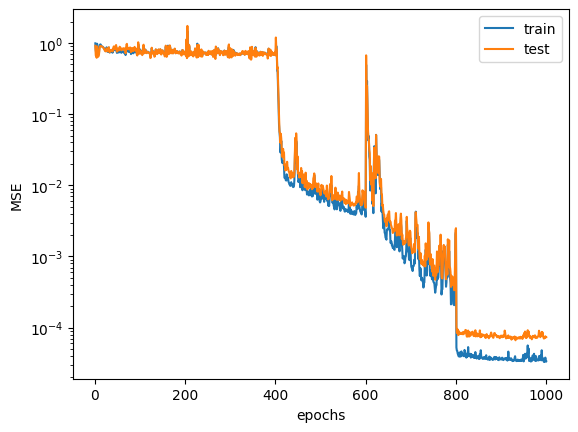
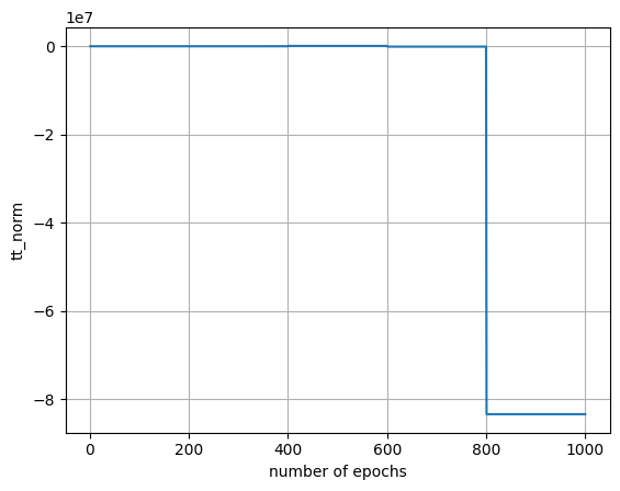
Results

Code

trace

shape: (1_000, 6)

epoch	mse_train	mse_test	mse_train_f	tt_norm	tt_ranks
i64	f64	f64	f64	f64	list[i64]
1	0.989216	0.913552	2.601824	1.0	[1, 1, … 1]
2	0.787074	0.670019	2.085504	1.0	[1, 1, … 1]
3	0.719287	0.653636	1.756305	1.0	[1, 1, … 1]
4	0.711022	0.620294	1.647353	1.0	[1, 1, … 1]
5	0.975683	0.895574	1.411286	1.0	[1, 1, … 1]
…	…	…	…	…	…
996	0.000035	0.000074	0.000101	-8.3396e7	[2, 2, … 2]
997	0.000033	0.000072	0.000099	-8.3396e7	[2, 2, … 2]
998	0.000038	0.000076	0.000102	-8.3396e7	[2, 2, … 2]
999	0.000034	0.000073	0.0001	-8.3396e7	[2, 2, … 2]
1000	0.000034	0.000074	0.000101	-8.3396e7	[2, 2, … 2]

Code

plt.plot(trace["epoch"], trace["mse_train"], label="train")
plt.plot(trace["epoch"], trace["mse_test"], label="test")
plt.xlabel("epochs")
plt.ylabel("MSE")
plt.yscale("log")
plt.legend()
plt.show()
trace.tail()

shape: (5, 6)

epoch	mse_train	mse_test	mse_train_f	tt_norm	tt_ranks
i64	f64	f64	f64	f64	list[i64]
996	0.000035	0.000074	0.000101	-8.3396e7	[2, 2, … 2]
997	0.000033	0.000072	0.000099	-8.3396e7	[2, 2, … 2]
998	0.000038	0.000076	0.000102	-8.3396e7	[2, 2, … 2]
999	0.000034	0.000073	0.0001	-8.3396e7	[2, 2, … 2]
1000	0.000034	0.000074	0.000101	-8.3396e7	[2, 2, … 2]

Code

plt.plot(trace["epoch"], trace["tt_norm"])
plt.xlabel("number of epochs")
plt.ylabel("tt_norm")
plt.grid()
plt.show()

Code

plt.plot(
    trace["epoch"],
    trace["tt_ranks"].to_list(),
    label=[f"M{i}" for i in range(n - 1)],
)
plt.legend()
plt.xlabel("epochs")
plt.ylabel("tt_ranks")
plt.grid()
plt.show()

Visualize 2D cut along equilibrium geometry

Before visualizing, we rescale model parameters to be consistent with the original scale because we trained with standardized data.

Code

nnmpo.rescale(x_scale, y_scale)

Code

import itertools

q0 = np.linspace(-1, 1, 100)
q1 = np.linspace(-1, 1, 100)
Q0, Q1 = np.meshgrid(q0, q1)

fig, ax = plt.subplots(n, n, figsize=(3 * n, 3 * n), dpi=300)
x = np.zeros((100 * 100, n))
x[:, 0] = Q0.flatten()
x[:, 1] = Q1.flatten()
y = ellipse_pes(x).reshape(Q0.shape)
im = ax[0, 0].contourf(Q0, Q1, y, 50, cmap="RdGy", vmax=9, vmin=0)
cbar_ax = fig.add_axes([0.92, 0.15, 0.02, 0.7])
fig.colorbar(im, cax=cbar_ax)
for dims in itertools.combinations(range(n), 2):
    x = np.zeros((100 * 100, n))
    x[:, dims[0]] = Q0.flatten()
    x[:, dims[1]] = Q1.flatten()
    y = nnmpo.forward(x).reshape(Q0.shape) + y_shift
    title = f"cut = {dims} pred"
    ax[dims[0], dims[1]].set_title(title)
    im = ax[dims[0], dims[1]].contourf(
        Q0, Q1, y, 50, cmap="RdGy", vmax=9, vmin=0
    )
for dims in itertools.combinations(range(n), 2):
    x = np.zeros((100 * 100, n))
    x[:, dims[0]] = Q0.flatten()
    x[:, dims[1]] = Q1.flatten()
    y = ellipse_pes(x).reshape(Q0.shape)
    title = f"cut = {dims} true"
    ax[dims[1], dims[0]].set_title(title)
    im = ax[dims[1], dims[0]].contourf(
        Q0, Q1, y, 50, cmap="RdGy", vmax=9, vmin=0
    )
for dim in range(n):
    ax[dim, dim].clear()
    x = np.zeros((100 * 1, n))
    x[:, dim] = q0
    y = nnmpo.forward(x).reshape(-1) + y_shift
    label = "pred" if dim == 0 else None
    ax[dim, dim].plot(q0, y, label=label)
    y = ellipse_pes(x).reshape(-1)
    label = "true" if dim == 0 else None
    ax[dim, dim].plot(q0, y, label=label)
    if dim == 0:
        ax[dim, dim].legend()

title = (
    f"Fitted with N={N}, M={max(trace['tt_ranks'][-1])}, "
    + f"loss={trace['mse_test'][-1]:.3e}"
)
fig.suptitle(title)
plt.savefig("data/6d_pes.png")
plt.show()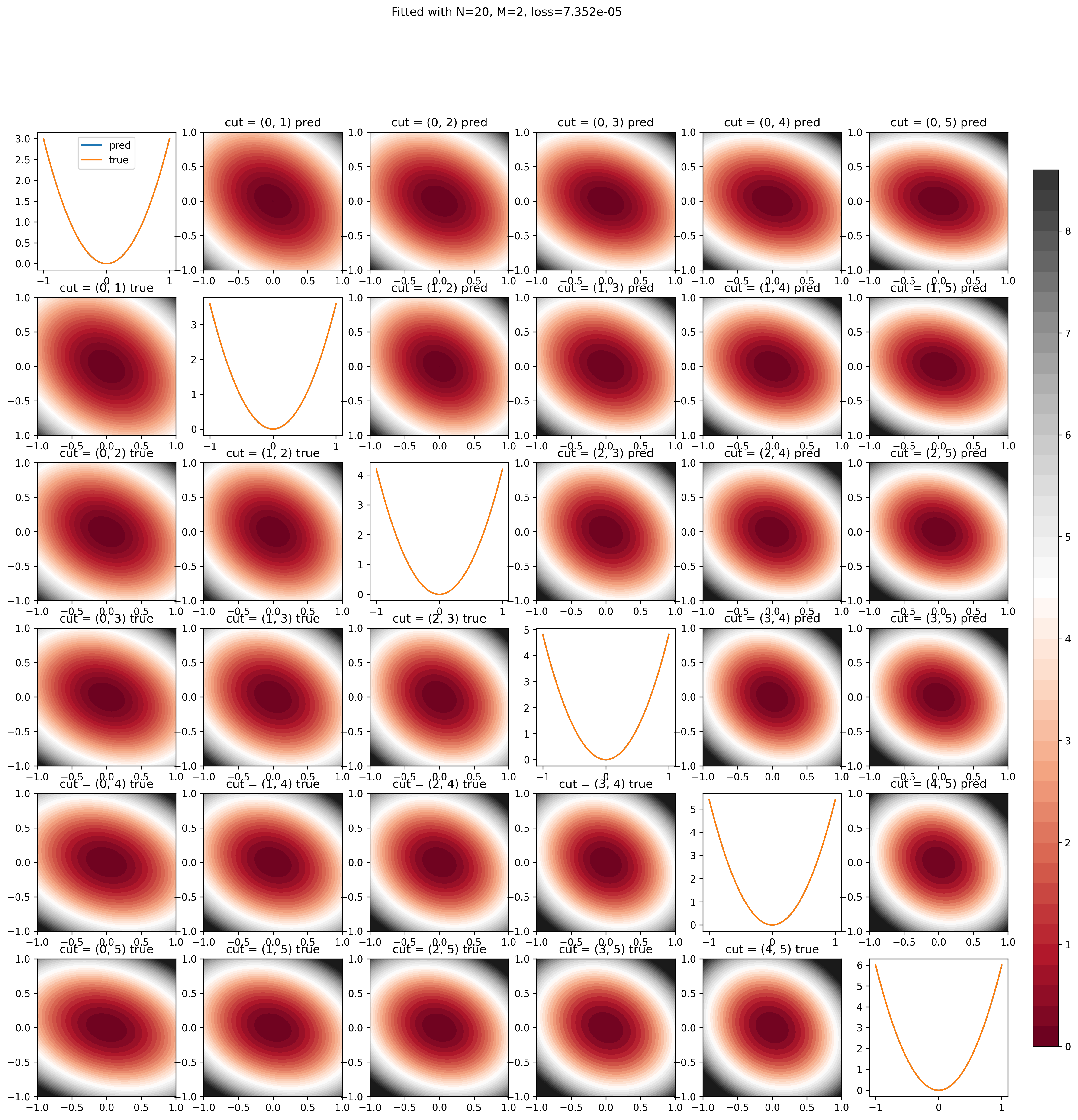

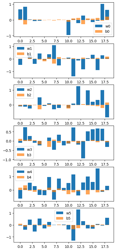
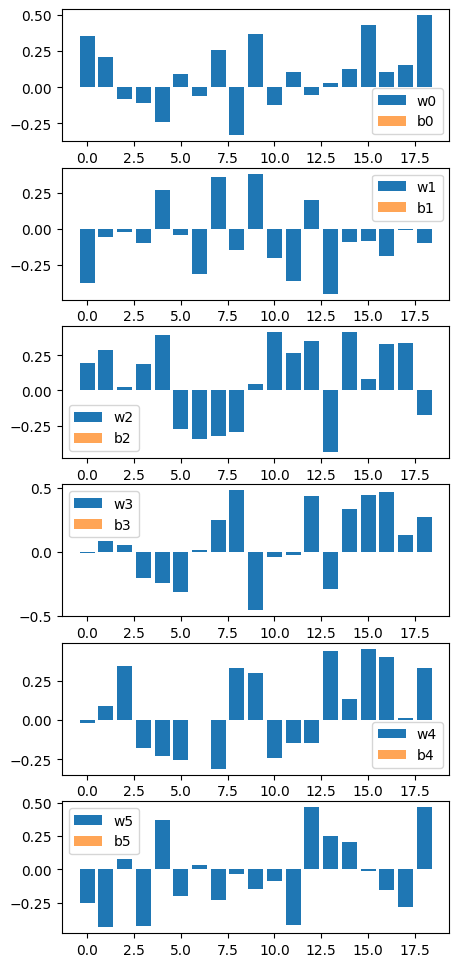
Visualize learning paramter. (chech over fitting occurs or not)

Code

nnmpo.basis.plot_data()

Code

show_basis(nnmpo)